Last step, calculate energy distribution and plot result.

By now, we have finished back-projection for waveforms. Next we need to summarize results back-projected from waveforms.

$ csh sum_energy.csh

# open sum_energy.csh to look over all commands

Duplicate

Read every grid’s stacked amplitudes.

# open mkcontour_max_smo-multi-V2.0.f to look over full commands

call system('ls stack.out > stackoutfiles')
  open (10, file='stackoutfiles')
      nth_BP = 0
      do
        read(10,'(a80)',iostat=iostat) ss; 
        if (iostat.ne.0) exit
        nth_BP = nth_BP + 1
    filename(nth_BP) = ss
      end do
close(10)

Smooth and normalize

# Open mkcontour_max_smo-multi-V2.0.f to view details

Calculate the maximun amplitude point

For every grid, calcaulte maximun amplitude point and corresponding point in time. And then, we obtain maximum spatial–temporal distribution of energy radiation.

Plot figure

As mentioned before, Back-projection of teleseismic P waves is a popular and efficient method to determine the rupture extent, duration and speed of large earthquakes. Usually we read these information directly by view figures.

$ csh Figure.4.gmt

# open Figure.4.gmt to look over all commands

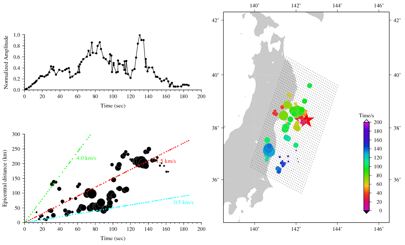
• (Top left) Normalized amplitudes varied with time. It’s obviously that there are two peaks, 70-90 s and 130 s and source duration can reach about 170 s.

• (Lower left) Distance-time display. The result show a variable rupture propagation ranging from about 0.5 to 3.0 km/s.

• (Right) Energy distribution in space and time. We can see two large pulses at 80 s and 130 s. The first was located about 60 km northwest of the epicenter and the other occurred about 250 km southwest of the epicenter.